This function plots discrete and continuous values results
Usage
mplot_density(
  tag,
  score,
  thresh = 6,
  model_name = NA,
  subtitle = NA,
  save = FALSE,
  subdir = NA,
  file_name = "viz_distribution.png"
)
Arguments
- tag
Vector. Real known label
- score
Vector. Predicted value or model's result
- thresh
Integer. Threshold for selecting binary or regression models: this number is the threshold of unique values we should have in 'tag' (more than: regression; less than: classification)
- model_name
Character. Model's name
- subtitle
Character. Subtitle to show in plot
- save
Boolean. Save output plot into working directory
- subdir
Character. Sub directory on which you wish to save the plot
- file_name
Character. File name as you wish to save the plot
See also
Other ML Visualization:
mplot_conf(),
mplot_cuts(),
mplot_cuts_error(),
mplot_full(),
mplot_gain(),
mplot_importance(),
mplot_lineal(),
mplot_metrics(),
mplot_response(),
mplot_roc(),
mplot_splits(),
mplot_topcats()
Examples
Sys.unsetenv("LARES_FONT") # Temporal
data(dfr) # Results for AutoML Predictions
lapply(dfr[c(1, 3)], head)
#> $class2
#> tag scores
#> 1 TRUE 0.3155498
#> 2 TRUE 0.8747599
#> 3 TRUE 0.8952823
#> 4 FALSE 0.0436517
#> 5 TRUE 0.2196593
#> 6 FALSE 0.2816101
#>
#> $regr
#> tag score
#> 1 11.1333 25.93200
#> 2 30.0708 39.91900
#> 3 26.5500 50.72246
#> 4 31.2750 47.81292
#> 5 13.0000 30.12853
#> 6 26.0000 13.24153
#>
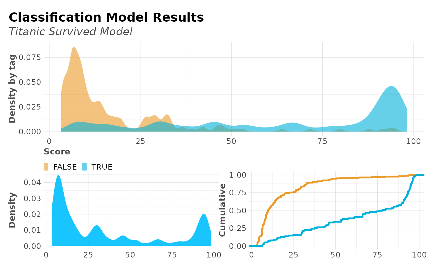
# Plot for binomial results
mplot_density(dfr$class2$tag, dfr$class2$scores, subtitle = "Titanic Survived Model")
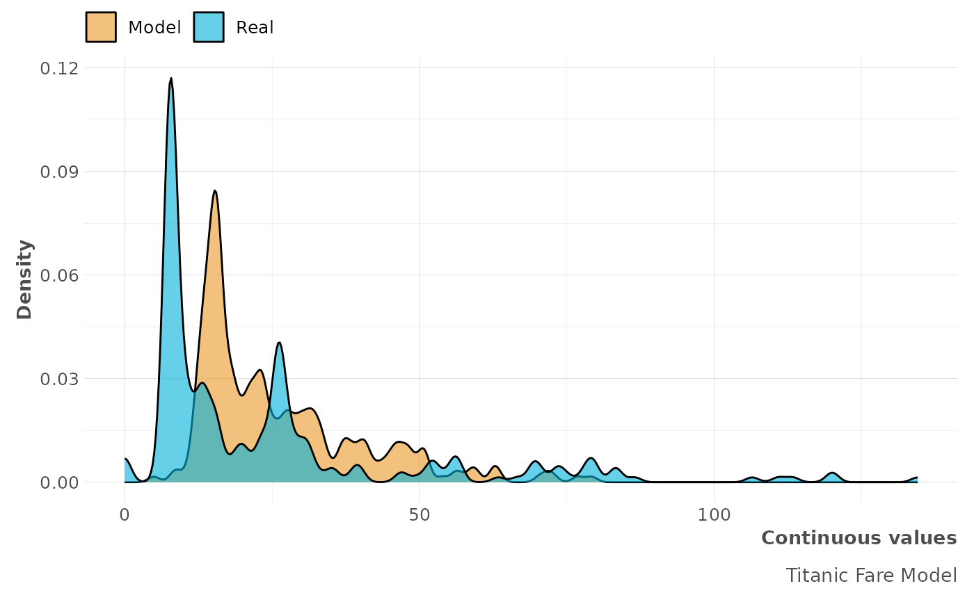
 # Plot for regression results
mplot_density(dfr$regr$tag, dfr$regr$score, model_name = "Titanic Fare Model")
# Plot for regression results
mplot_density(dfr$regr$tag, dfr$regr$score, model_name = "Titanic Fare Model")