The cumulative gains plot, often named ‘gains plot’, helps us answer the question: When we apply the model and select the best X deciles, what expect to target? The cumulative gains chart shows the percentage of the overall number of cases in a given category "gained" by targeting a percentage of the total number of cases.
Usage
mplot_gain(
  tag,
  score,
  multis = NA,
  target = "auto",
  splits = 10,
  highlight = "auto",
  caption = NA,
  save = FALSE,
  subdir = NA,
  file_name = "viz_gain.png",
  quiet = FALSE
)
Arguments
- tag
Vector. Real known label.
- score
Vector. Predicted value or model's result.
- multis
Data.frame. Containing columns with each category probability or score (only used when more than 2 categories coexist).
- target
Value. Which is your target positive value? If set to 'auto', the target with largest mean(score) will be selected. Change the value to overwrite. Only works for binary classes
- splits
Integer. Numer of quantiles to split the data
- highlight
Character or Integer. Which split should be used for the automatic conclussion in the plot? Set to "auto" for best value, "none" to turn off or the number of split.
- caption
Character. Caption to show in plot
- save
Boolean. Save output plot into working directory
- subdir
Character. Sub directory on which you wish to save the plot
- file_name
Character. File name as you wish to save the plot
- quiet
Boolean. Keep quiet? If not, informative messages will be shown.
See also
Other ML Visualization:
mplot_conf(),
mplot_cuts(),
mplot_cuts_error(),
mplot_density(),
mplot_full(),
mplot_importance(),
mplot_lineal(),
mplot_metrics(),
mplot_response(),
mplot_roc(),
mplot_splits(),
mplot_topcats()
Examples
Sys.unsetenv("LARES_FONT") # Temporal
data(dfr) # Results for AutoML Predictions
lapply(dfr, head)
#> $class2
#> tag scores
#> 1 TRUE 0.3155498
#> 2 TRUE 0.8747599
#> 3 TRUE 0.8952823
#> 4 FALSE 0.0436517
#> 5 TRUE 0.2196593
#> 6 FALSE 0.2816101
#>
#> $class3
#> tag score n_1 n_2 n_3
#> 1 n_3 n_2 0.20343865 0.60825062 0.18831071
#> 2 n_2 n_3 0.17856154 0.07657769 0.74486071
#> 3 n_1 n_1 0.50516951 0.40168718 0.09314334
#> 4 n_3 n_2 0.30880713 0.39062151 0.30057135
#> 5 n_2 n_3 0.01956827 0.07069011 0.90974158
#> 6 n_2 n_3 0.07830017 0.15408720 0.76761264
#>
#> $regr
#> tag score
#> 1 11.1333 25.93200
#> 2 30.0708 39.91900
#> 3 26.5500 50.72246
#> 4 31.2750 47.81292
#> 5 13.0000 30.12853
#> 6 26.0000 13.24153
#>
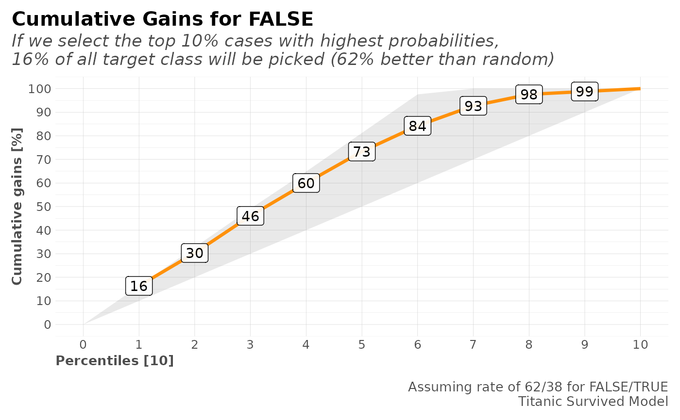
# Plot for Binomial Model
mplot_gain(dfr$class2$tag, dfr$class2$scores,
caption = "Titanic Survived Model",
target = "FALSE"
)
#> Target value: FALSE
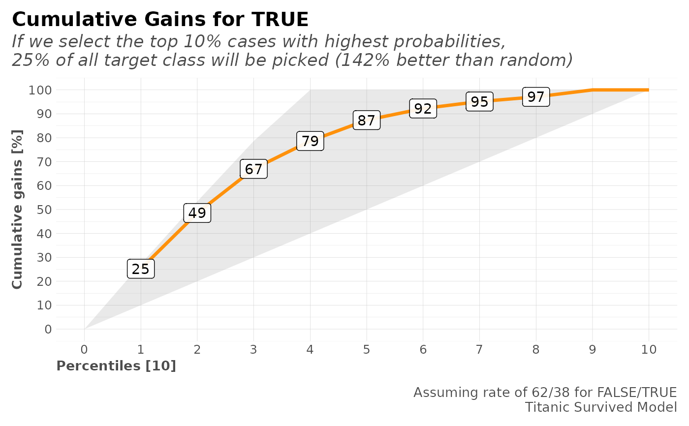
 mplot_gain(dfr$class2$tag, dfr$class2$scores,
caption = "Titanic Survived Model",
target = "TRUE"
)
#> Target value: TRUE
mplot_gain(dfr$class2$tag, dfr$class2$scores,
caption = "Titanic Survived Model",
target = "TRUE"
)
#> Target value: TRUE
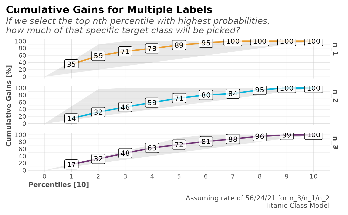
 # Plot for Multi-Categorical Model
mplot_gain(dfr$class3$tag, dfr$class3$score,
multis = subset(dfr$class3, select = -c(tag, score)),
caption = "Titanic Class Model"
)
#> Target value: n_1
#> Target value: n_2
#> Target value: n_3
#> Ignoring unknown labels:
#> • linetype : "Reference"
# Plot for Multi-Categorical Model
mplot_gain(dfr$class3$tag, dfr$class3$score,
multis = subset(dfr$class3, select = -c(tag, score)),
caption = "Titanic Class Model"
)
#> Target value: n_1
#> Target value: n_2
#> Target value: n_3
#> Ignoring unknown labels:
#> • linetype : "Reference"