Correlation between variable and dataframe

This function correlates a whole dataframe with a single feature. It automatically runs ohse (one-hot-smart-encoding) so no need to input only numerical values.

Usage

corr_var(
  df,
  var,
  ignore = NULL,
  trim = 0,
  clean = FALSE,
  plot = TRUE,
  top = NA,
  ceiling = 1,
  max_pvalue = 1,
  limit = 10,
  ranks = FALSE,
  zeroes = FALSE,
  save = FALSE,
  quiet = FALSE,
  ...
)

# S3 method for class 'corr_var'
plot(x, var, max_pvalue = 1, top = NA, limit = NULL, ...)

Arguments

df: Dataframe. It doesn't matter if it's got non-numerical columns: they will be filtered.
var: Variable. Name of the variable to correlate. Note that if the variable var is not numerical, 1. you may define which category to select from using `var_category`; 2. You may have to add redundant = TRUE to enable all categories (instead of n-1).
ignore: Character vector. Which columns do you wish to exclude?
trim: Integer. Trim words until the nth character for categorical values (applies for both, target and values)
clean: Boolean. Use lares::cleanText for categorical values (applies for both, target and values)
plot: Boolean. Do you wish to plot the result? If set to TRUE, the function will return only the plot and not the result's data
top: Integer. If you want to plot the top correlations, define how many
ceiling: Numeric. Remove all correlations above... Range: (0-1]
max_pvalue: Numeric. Filter non-significant variables. Range (0, 1]
limit: Integer. Limit one hot encoding to the n most frequent values of each column. Set to NA to ignore argument.
ranks: Boolean. Add ranking numbers?
zeroes: Do you wish to keep zeroes in correlations too?
save: Boolean. Save output plot into working directory
quiet: Boolean. Keep quiet? If not, show messages
...: Additional parameters passed to corr and cor.test
x: corr_var object

Value

data.frame. With variables, correlation and p-value results for each feature, arranged by descending absolute correlation value.

Examples

Sys.unsetenv("LARES_FONT") # Temporal
data(dft) # Titanic dataset

corr_var(dft, Survived, method = "spearman", plot = FALSE, top = 10)
#> Warning: Not a valid input: Survived was transformed or does not exist.
#>   >> Automatically using 'Survived_TRUE'
#> # A tibble: 10 × 3
#>    variables      corr   pvalue
#>    <chr>         <dbl>    <dbl>
#>  1 Sex_male     -0.543 1.41e-69
#>  2 Fare          0.324 3.47e-23
#>  3 Pclass_3     -0.322 5.51e-23
#>  4 Cabin_       -0.317 3.09e-22
#>  5 Pclass_1      0.286 3.19e-18
#>  6 Cabin_OTHER   0.278 2.95e-17
#>  7 Embarked_C    0.168 4.40e- 7
#>  8 Embarked_S   -0.156 3.04e- 6
#>  9 Parch         0.138 3.45e- 5
#> 10 Ticket_OTHER  0.103 2.17e- 3

# With plots, results are easier to compare:

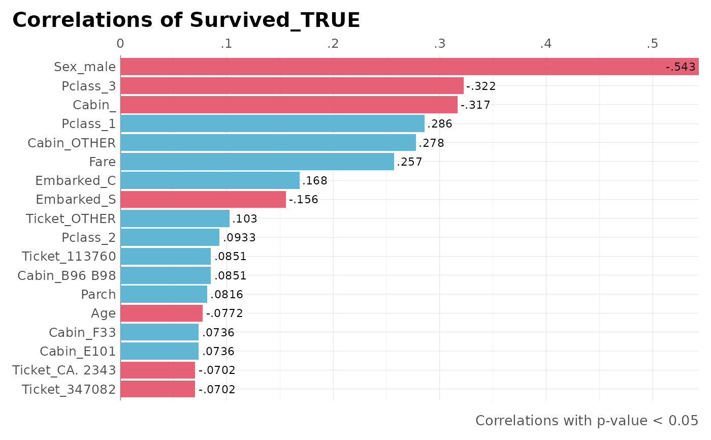
# Correlate Survived with everything else and show only significant results
dft %>% corr_var(Survived_TRUE, max_pvalue = 0.05)


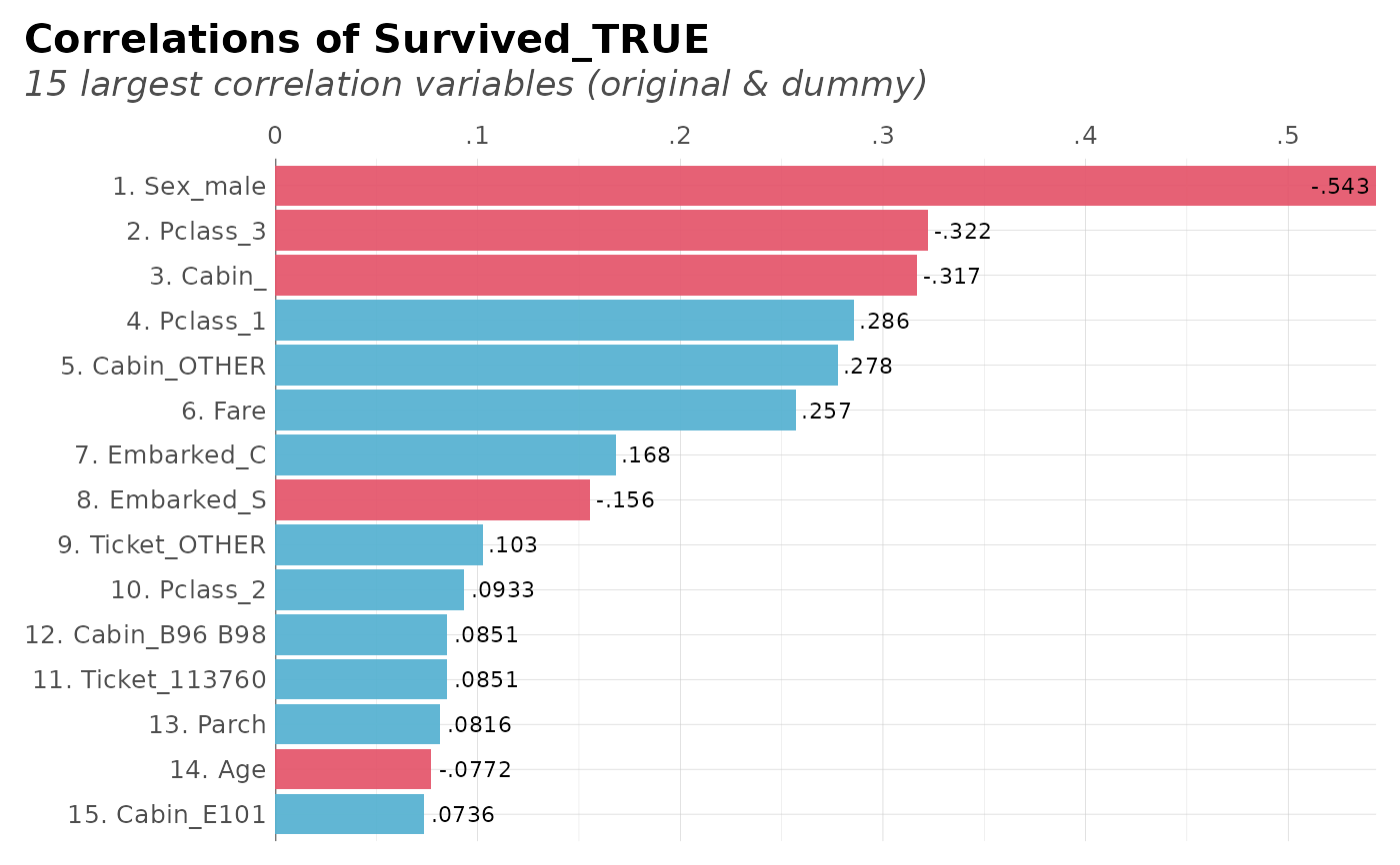
# Top 15 with less than 50% correlation and show ranks
dft %>% corr_var(Survived_TRUE, ceiling = .6, top = 15, ranks = TRUE)
#> Removing all correlations greater than 60% (absolute)

Correlation between variable and dataframe

Usage

Arguments

Value

See also

Examples